Intro
What is dynamic programming?
it refers to simplifying a complicated problem by breaking it down into simpler sub-problems in a recursive manner
This might sound rather vague and a bit intimidating. My definition?
careful brute force
In class we are used to learning about all sorts of algorithms like binary search where memorization of the algorithm can be favored in exchange of understanding the underlying concept. Often times, I hear my friends growl whenever we bump into a DP/recursion problem while doing interview prep. I hope that with this article I can shed some light behind dynamic programming and teach you how you can intuitively deconstruct a problem and solve it!
Fibonacci Sequence
There’s no better way to explain DP than using the Fibonacci Sequence. To give you a quick refresher, the sequence is constructed such that each number is the sum of the two preceding ones.


Recursive Implementation
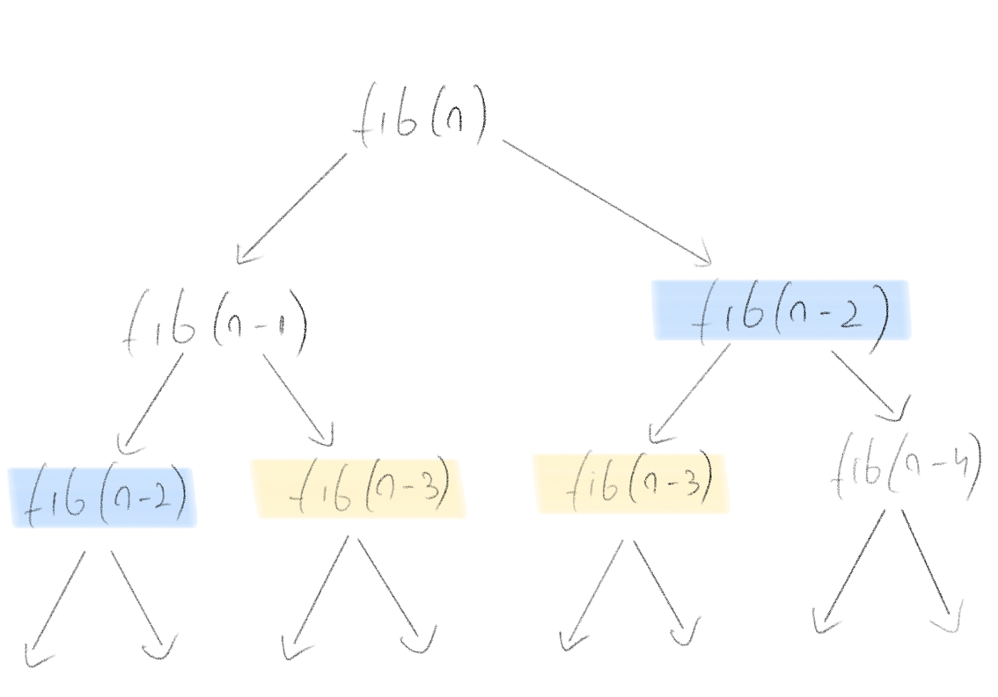
The first step to DP is to figure out sub-problems. We are going to take a top-down approach where we break the initial problem into smaller and smaller subproblems that become effectively easier to solve. In the case of Fibonacci, we will start with the number we want to find and trickle our way downwards to the base case, which is the first two elements of the sequence, 1 & 1.
I’ve took the liberty and implemented the aforementioned solution in python.
def fib(n):
  if n <= 2:
    return 1
  else:
    return fib(n - 1) + fib(n - 2)
It looks fairly straightforward, right?
Before we move any further, we need to take a step back and analyze the time complexity or as it is called in this case, the recurrence. This can be rather tricky to calculate, therefore approximating the result is perfectly fine.


Hmm 🤔, looks like the fib function has exponential time. Let me explain! The problem is that we end up calculating a bunch of the same values multiple times.

Memoized Recursive Implementation
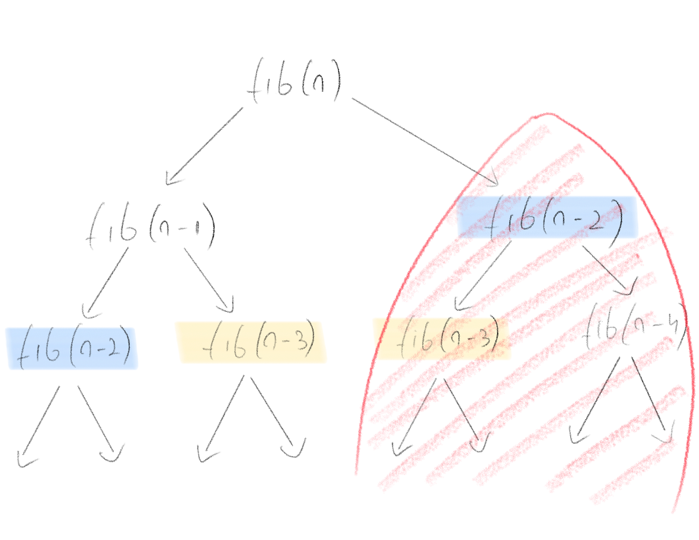
The beauty of DP is that it can shrink down the exponential time complexity of a brute force algorithm to polynomial (≈ linear) time. The second step of DP is to memoize and reuse those subproblems.
Going back to our fib implementation this is fairly easy to implement by using a dictionary that will keep track of solutions that have been already solved.
memo = {}
def fib(n):
  if n in memo:
    return memo[n]
  if n <= 2:
    f = 1
  else:
    f = fib(n - 1) + fib(n - 2)
  memo[n] = f
  return f
Now, calculating the time complexity comes down to multiplying the number of subproblems by the amount of time per subproblem (no need to count memoized solutions). This quick optimization reduced the complexity from exponential time to linear time, O(n). We have n subproblems (n fibonacci numbers that we need to calculate and for each one of them it takes O(1) to compute.
time complexity = subproblems * (time complexity / subproblem)

Iterative Implementation
Some people prefer to take an iterative approach instead of recursion. Everyone has their own style of solving problems and writing code, so I also wanted to briefly mention the iterative solution for DP. In this case, you would want to take a bottom-up approach and create a DP table that will memoize the previous solutions.
In this implementation of fib I’m only memoizing the last 2 numbers of the sequence since that is all we need.
def fib(n):
  a, b = 1, 1

  for i in range(n):
    a, b = b, a + b

  return a
Conclusion
To sum up DP in 5 “easy steps” here’s the battle tested approach that will work for any problem:
- define and split into subproblems
- guess part of the solution (this will only become more clear with time)
- relate subproblems
- recurse and memoization (reuse subproblems)
- solve original problem
I hope that from now on you will approach DP problems with joy and excitement!
Citations
This article wouldn’t have been possible without the following materials: